


Introduction:
The US Tax Credit and IRA-Ready Financial Model for Renewable Projects is an invaluable template designed for individuals seeking to evaluate the returns of renewable energy projects accounting for all the tax credits and incentives available in the USA, such as:
- Incentive Tax Credit
- Production Tax Credit
- Investment Based Incentive
- Capacity Based Investment
- Production Based Investment
- Bonus Depreciation
- Federal and State Taxes
With this model, you can determine:
- Equity Internal Rate of Return (IRR),
- Net Present Value (NPV),
- Levelized Cost of Electricity (LCoE)
This financial model is tailored for individuals seeking a clear and user-friendly method to analyze renewable energy projects, with a specific emphasis on projects based in the USA. |
The model is divided into the following sheets:
- Inputs
- Cash Flow
- Debt
- Tax
- Incentives
- ITC
- Depreciation Calculations
- Depreciation Schedules
- Reserve Accounts
- Technical
- Timeline
Certainly! If you want to integrate the round button code into your existing HTML, you can use the following: html Copy code
The Model Inputs:
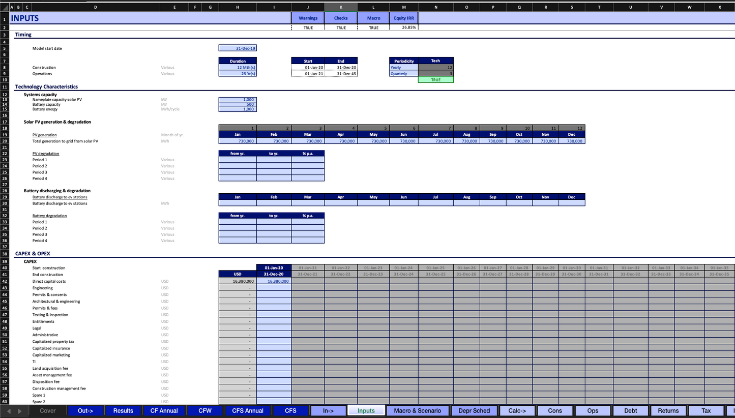
Period of Analysis: The number of years the analysis will run for.
Generation: The model allows the user to set the different values for generation per year in kWh and the in depreciation of the generation as %/year for different periods.
In the example above, the generation is set for:
- 876,000 KWh per year from years 1 to 10 with a degradation of 1%year
- 880,00 KWh per year from years 11 to 21 with a degradation of 1%year, and
- 875,000 KWh per year from years 21 to 30 with a degradation of 1%year.
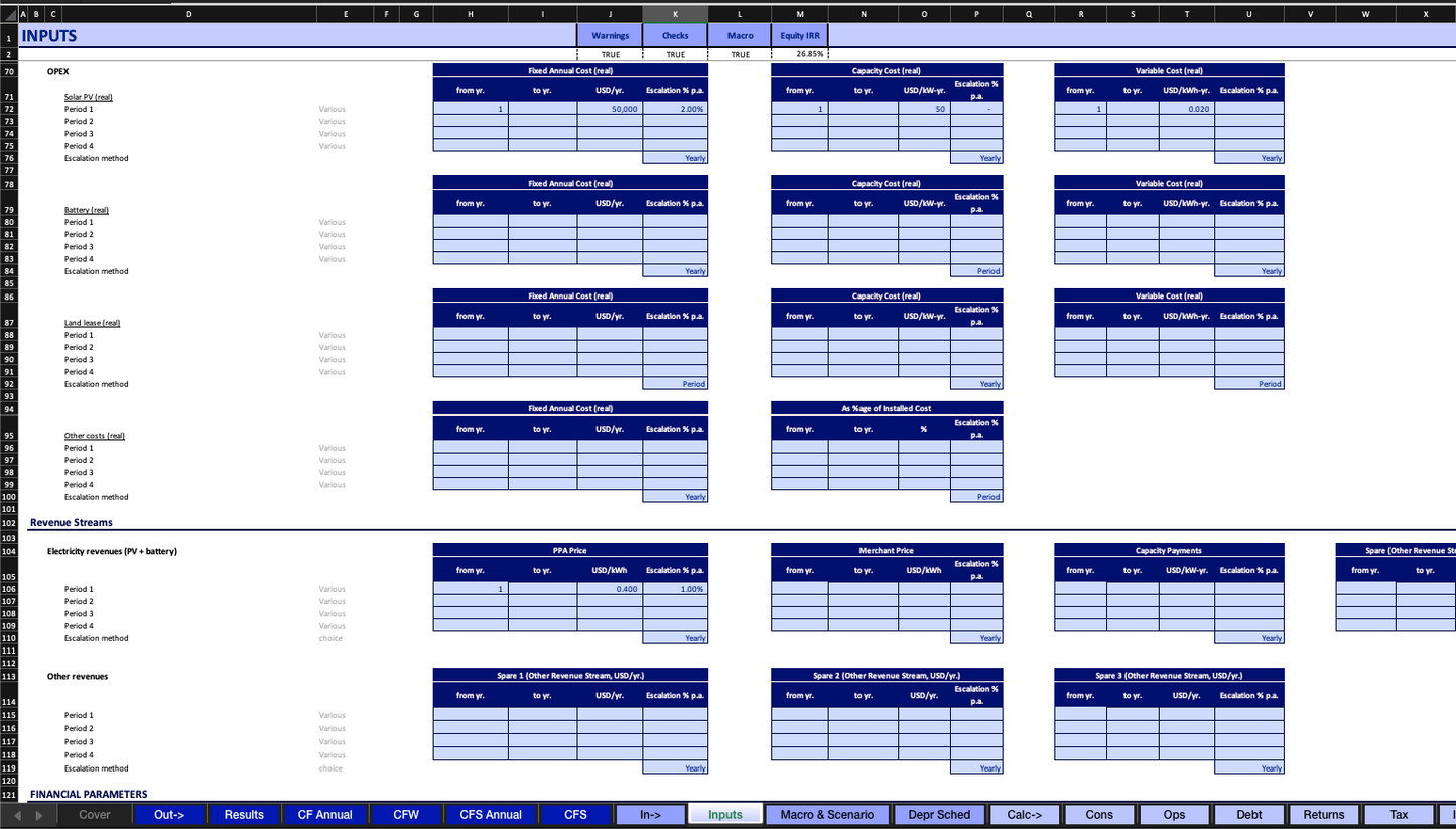
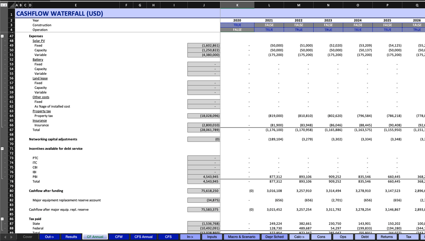
CAPEX & OPEX:
These can be added to the model as a function of:
- Fixed cost per year: USD
- Based on the installed capacity: USD/kW
- Based on the energy produced: USD/kWh
The OPEX can also be broken down in different periods and have individual escalations.
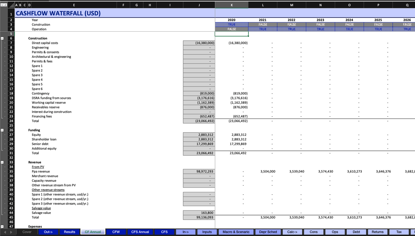
Revenues: The inputs for the revenues are shown in the figure below.
The "Other Revenues" fields are added individually for each one of the years.
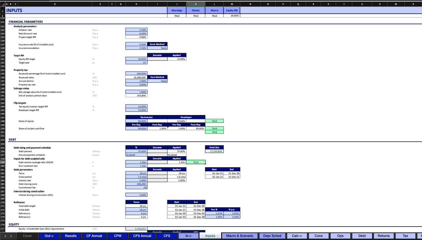
Financial Parameters: Inflation, Insurances, property tax, and salvage values are the inputs of this sheet.
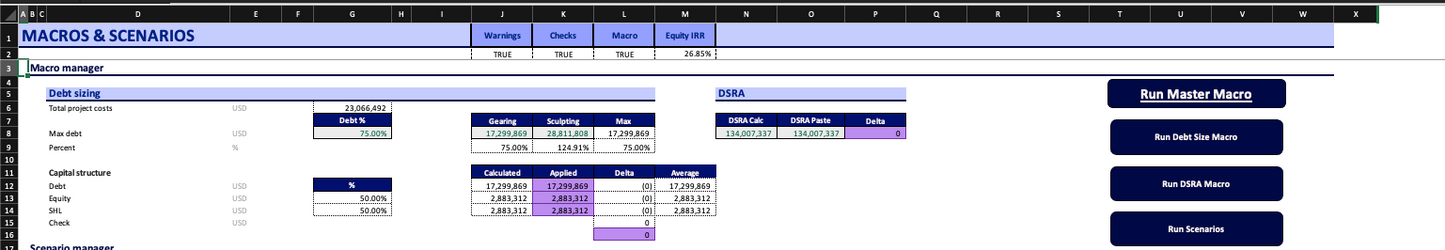
Debt: The model offers flexibility in determining the size of debt, allowing you to choose between two methods:
Percentage of Total Installed Cost:
Specify the debt size as a percentage of the total installed cost, inclusive of any additional fees and incentives. The annual debt-service coverage ratio (DSCR) varies from year to year.
Debt-Service Coverage Ratio (DSCR) & Debt Sculpted:
Specify the desired DSCR, and let the model calculate the debt size based on the annual cash available for debt service from the project cash flow. This approach ties the size of debt to annual revenue and operating costs rather than the total installed cost.
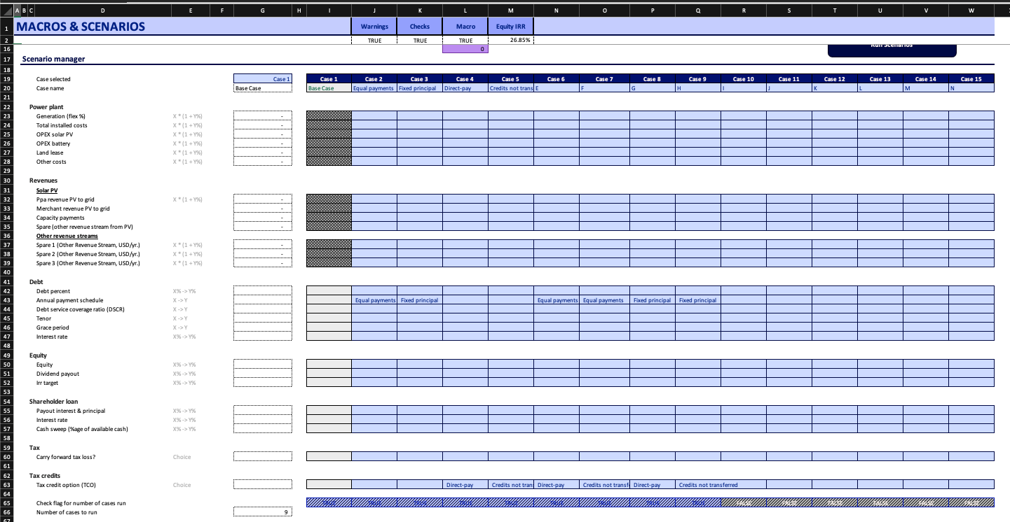
Amortization Methods: When the percentage of total installed costs is activated, there is the possibility to pay the principal either through:
- Equal Payments: debt payments constant over the tenor of the debt
- Fixed Principal, declining interest: constant principal payment size and reducing annual interest payment.
Construction Financing Calculation: To prevent circularity in the model and eliminate reliance on macros, the assumption governing the model posits that the entire construction balance remains outstanding for half of the construction period. This assumption aligns with a uniform monthly draw schedule, thereby yielding an average loan life equivalent to half of the construction period. If you need to simulate a different draw schedule, you have the option to adjust the loan's interest rate accordingly.
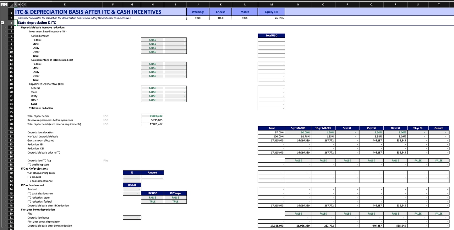
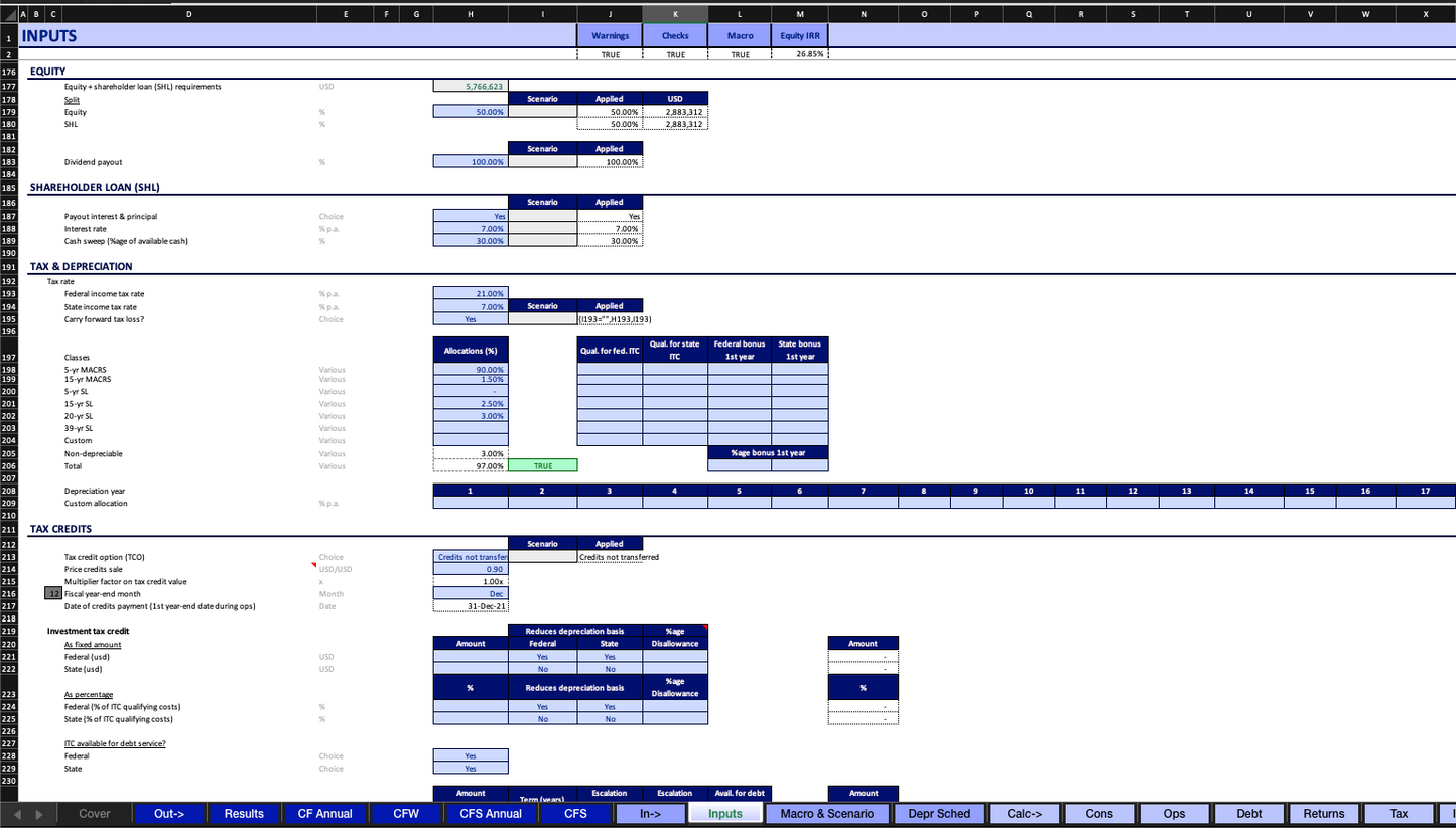
Tax & Depreciation: For tax, the user can input federal and state tax percentages.
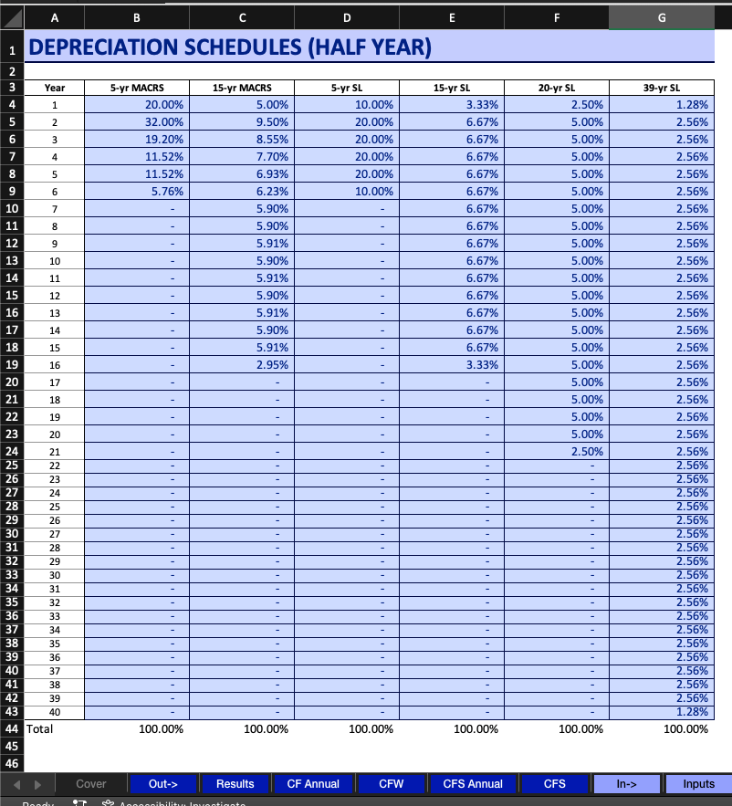
In the depreciation section, users can choose from various commonly utilized depreciation schedules in the USA, such as:
- MACRS 5 & 15 years
- Straight Line 5, 15, 20, 39 years
If you need a specific depreciation, you can use the "Custom" input and define a schedule in %/year as per your requirements.
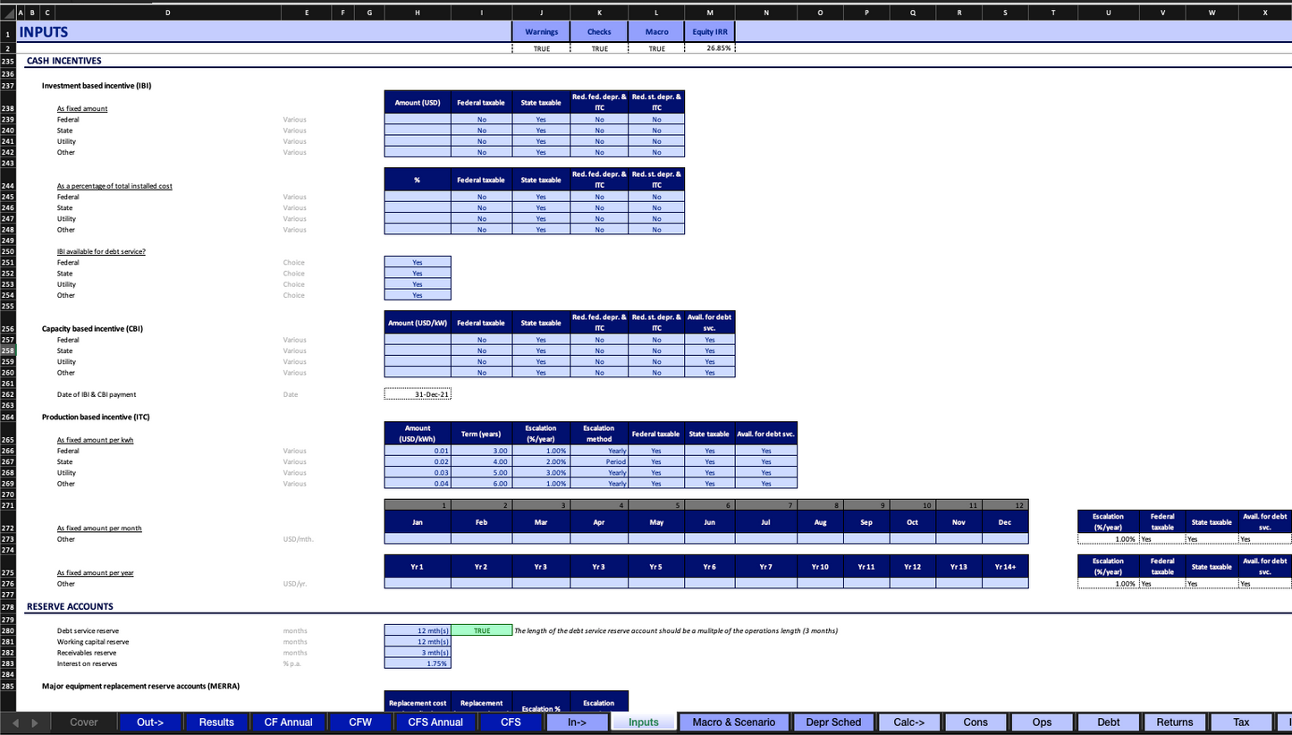
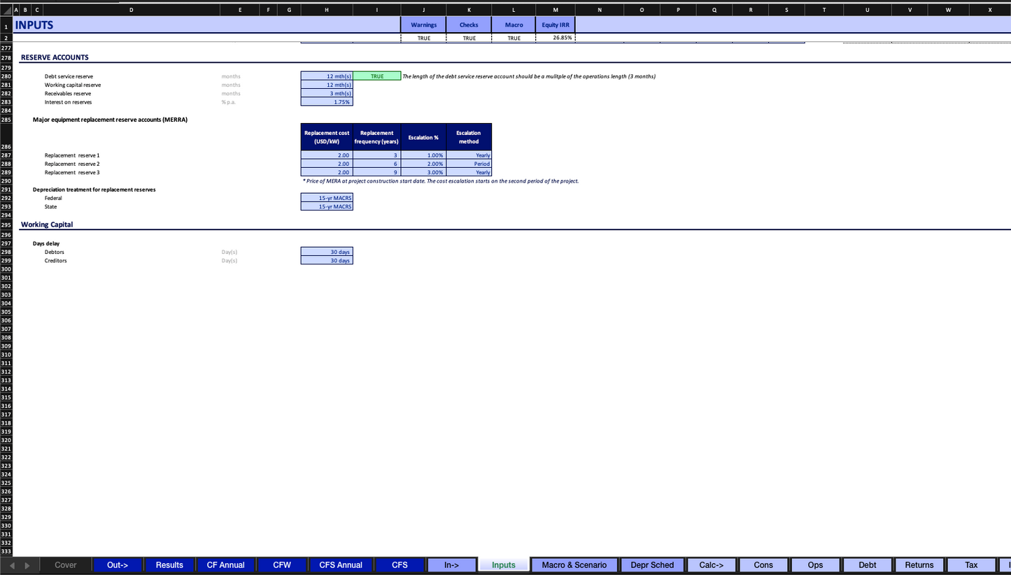
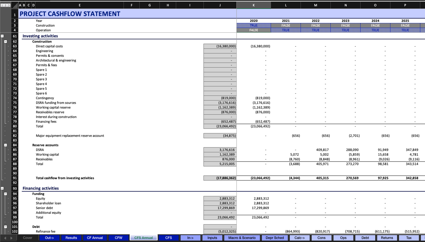
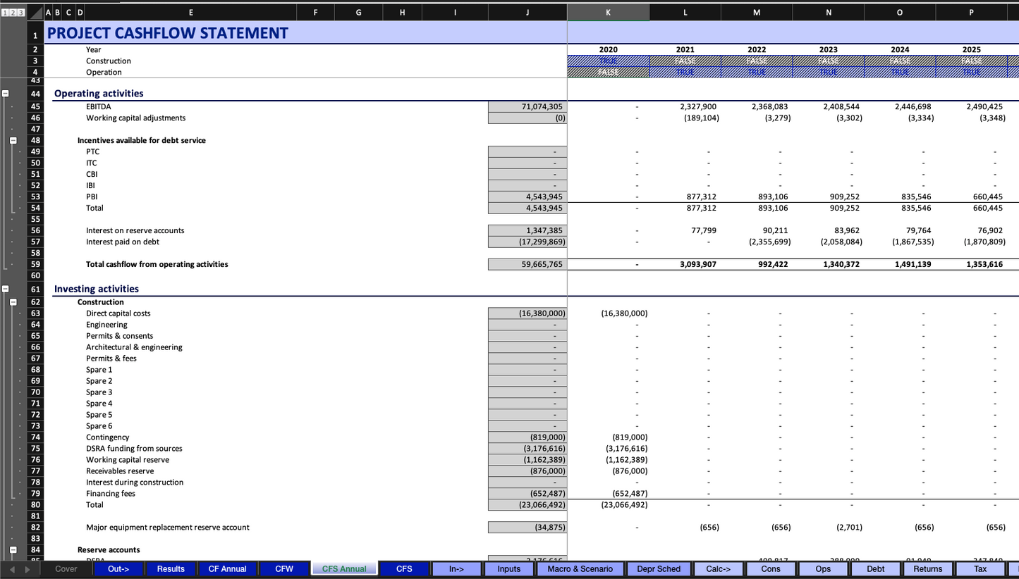
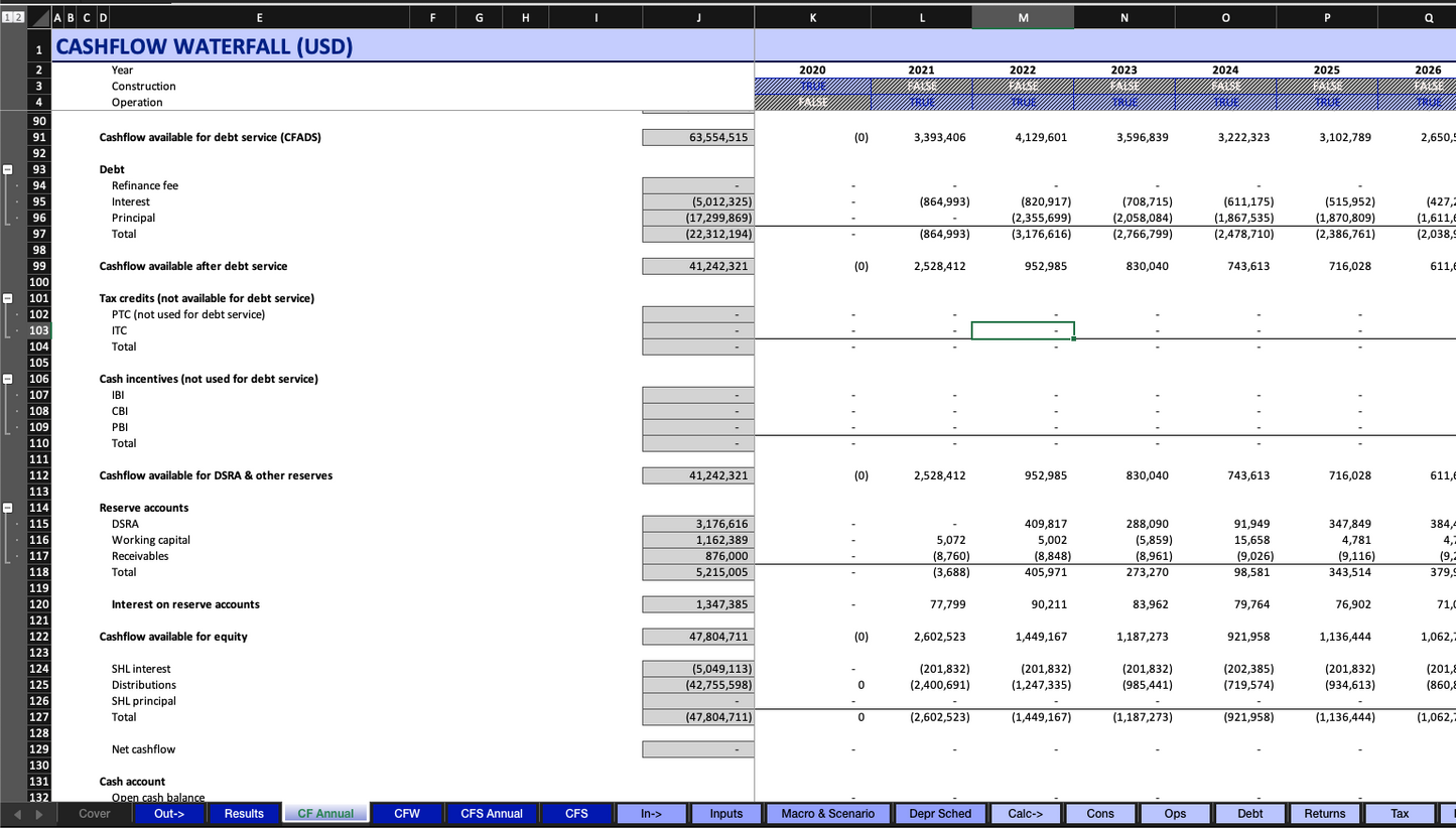
Reserve Accounts: The model has the following reserve accounts available:
- Working Capital
- Major Replacement Account
Tax Credits: Investment & Production Tax Credit at Federal and State levels.
Direct Cash Incentives: Investment Based Incentives, Capacity Based Incentive and Production Based Incentives.
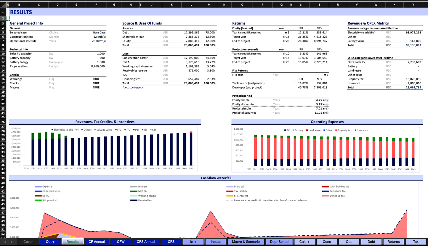
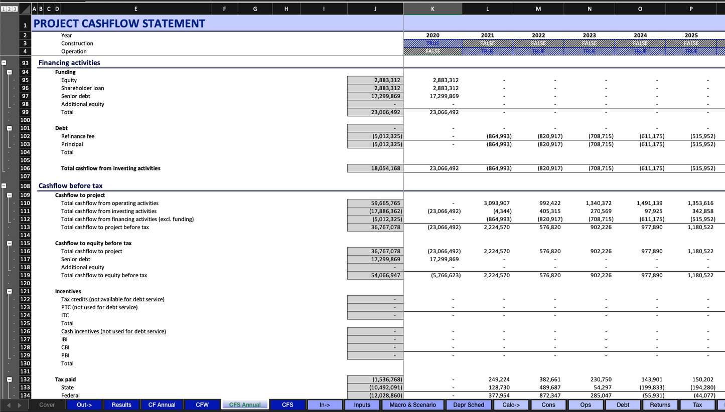
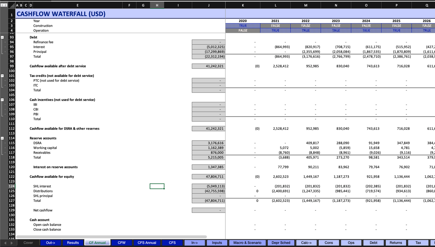
The Model Results:
The outcome of the model are presented in the sheet Cash Flow as Equity IRR and NPV, LCoE, and LPPA.